TAM is defined as the revenue a company could realized while having 100 per cent market share while creating shareholder value. The ability to calibrate the total addressable market (TAM) is a major part of anticipating value creation.

This report provides a framework for estimating TAM through the process of triangulation. Three methods are used – first is based on population, product and conversion. Next diffusion model is analyzed in which addresses absolute size of market and also rate of adoption. Finally, base rate check is done for reality check.

Categorizing New Products

To assess market size categorization of product is a logical starting point. This allows us to appraise a company’s strategy to promote the product. Companies can influence their TAM through pricing strategy and product enhancement. Pricing strategy is when companies sell products at discount in order to gain market share. Product enhancement can reflect improvement in the product itself.

Current technologies that have applications for new customers and new technologies used by current customers are the categories where a TAM analysis is most relevant. TAM is tricky to analyze when both technology and customers are new.

Some specific ways to estimate TAM –

Market Size – Population, Product and Conversion

First approach is to estimate absolute market size, in which number of potential customers is multiplied with expected revenue per customer. There are three parts for this analysis – first is population in which we estimate the population which can use our product, second is product in which we estimate population which is likely to use our product and the last is conversion where we analyze what can be the potential revenue. Factors that shape up demand and supply can be considered for doing more in – depth analysis of absolute market size.

Factors to consider in assessing demand are financial resources, physical limitations, elasticity of demand, cyclicality, substitution and substitution threats.

Factors to consider in assessing supply are ability to supply, unit growth and pricing, regulatory constraints, incentives, scale, niches.

TAM and the Bass Model

The Bass model allows for a prediction of the purchasers in a period, say for each year, as well as a total number of purchasers. Bass model relies on three parameters –

1. The coefficient of innovation (p) – This captures mass-market influence
2. The coefficient of imitation (q) – This reflects interpersonal influence.
3. An estimate of the number of eventual adopters (m) – A parameter that determines the size of the market.

The equation for the Bass model is – N(t) – N(t−1) = [p + qN(t−1)/m] x

This formula simply says that new adopter’s equal the adoption rate multiply the number of potential new adopters.

N(t) – N(t−1) shows the number of adopters during a period i.e. simply the difference between the users now, N(t), and the users in the prior period, N(t−1). First term on the right side of the equation spells out the rate of adoption. The second term on the right side is the number of users who have not yet adopted the product.

Investor application of the Bass model –

The first is to estimate product potential based on the parameters from historical diffusions. Second way to use the model is to start with a company’s stock price and backwards.

Bass model also allows solving for the size of peak sales. For calculating the size of peak sales this equation can be used –

Size of peak sales = m[(p+q)² / 4q].

There are typically three stages in industry evolution. During the first stage, the number of competitors grows. In second stage there are large shakeouts as the result of higher number of firms exiting. In third stage, number of competitors and market shares stabilizes. In stage two company’s sales can grow faster as the numbers of competitors are reducing.

Limitations for Bass model –

This model can be helpful in judging TAM. But there are some limitations that don’t allow it to capture certain considerations.

First limitation is of replacement cycle. Bass model is used primarily for forecasting adoption of a product. But very less attention is given to replacement cycle. Replacement cycle talks about replacement of a product once the purchase is done.

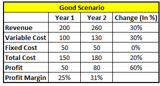
Second limitation is of economies of scale. Economies of scale is when company’s fixed cost gets spread over higher sales i.e. when company do more sales then the fixed cost spreads over a larger base. This limits the level of TAM because companies fail to create value after a certain size. There is a separate issue with similar implications. This is when companies overshoot their markets. Two symptoms of overshot market are customers use only a fraction of the functionally the product offers and they are not paying for new features.

Third limitation is of network effect. Network effect is there when value of one product increases when more people start using it. Example – telephone. If only one person is using then it has very little value. But as more number of people starts using it the value increases. In businesses where strong network effect is there, market shares of companies are higher. Companies spend heavily in the hope that their product will become the product of choice but in sectors with strong network effects, most companies fail to go from early adopters to mainstream users.

Base rates as a reality check –

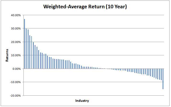
Third method in the triangulation process to estimate TAM is careful consideration of base rates. The main idea is to refer to what happened to other companies when they were in the same stage. This can be useful because, say for example, a company’s management is saying that they can grow at 10% CAGR in the coming 5 years. But in base rate method we check that what happened to other companies when they were in the same stage. This can be a reality check. Base rates provide a check on the output of the first two approaches to estimating TAM.

TAM and Ecosystems

Generally business can be in three categories – Physical, Service and Knowledge. Main objective is to understand the characteristics of these categories and to consider how companies can expand across them.

Physical – Main source of cash flow for these businesses is tangible assets like manufacturing facilities, stores and inventory etc. Sales growth is tied to asset growth.

Service – Main source of competitive advantage is people for service businesses.

Knowledge – These businesses also rely on people as their main source of competitive advantage.

These categories differ in economic characteristics. Some considerations are as –

Source of advantage – Physical companies depend on tangible assets while service and Knowledge business depend on people.

Investment trigger – Physical and service business can grow by adding capacity either in the form of CAPEX or new employees. Knowledge businesses generally invest to deal with obsolescence.

Products and Protecting Capital – Rival goods are those where consumption of one’s product will decrease the consumption of others. Non-rival goods are generally difficult to protect because they are relatively easy and cheap to replicate. Creator of a non-rival good often has difficulty capturing the value. One strategy companies use to increase TAM is to extend business in new business categories. This extension can have challenges such as trade-offs between open and closed systems, functionality in the product or in the cloud, determining which party owns the data, and whether or not to monetize data by selling to outside parties.  

This research paper discusses about value migration in 4 industries.

What is value migration?

Value migration is flow of economic value from old business model to new business model which are better able to satisfy customers. For example – Shifting of people from black and white television to colour television was value migration. For colour television industry it was value inflow but for black and white television industry it was value outflow.

Value migration happens in three stages –

Value Inflow – Companies or Industry is able to capture value from other industries or companies due to superior value.

Stability – Competitive equilibrium is established.

Value Outflow – Value move towards new industry or industry which are better able to cater needs of customers.

The four sectors covered in this paper are BFSI, Information technology, Oil and Gas, Consumer (Jewelry)

BFSI –

Shift is happening from public sector banks to private sector banks which are customer friendly. Corporate banking sector is facing challenges and public sector banks will face challenges on capitalization and growth. While private sector banks can emerge stronger because they have used digital capabilities and also expanded their branch network. They also have a strong traction in CASA mix.

Private sector banks have invested heavily in technology and have come up with various innovative products. Their CASA grew at fast pace. Also private sector banks have good digital architecture. They have higher share in digital transactions. Private sector banks have taken balanced approach. Through strategic partnership costs are under control and also profitability has been maintained.

For public sector banks, government announced recapitalization plan but most of the money will be used in provisioning requirement. FY 19 was in full compliance with Basel –III regulations; there was pressure on public sector banks to meet the capital norms.

Thus, value migration is accelerating in BFSI.

IT –

In last decade, Indian IT industry was in high growth trajectory. It was driven by cost – led value migration. But industry reached the stability phase once the market share gains and profit margins started to settle. But now the changing priorities are clearly visible. Next level of savings is offered by automation which will make location irrelevant. Client’s technology systems are changing. Digital transformation is needed to survive threat from born in cloud organizations. Indian IT industry needs to replace traditional stream revenue with new ones.

Oil and Gas –

In recent years, rising pollution is a key concern while making policies. According to WHO, half of the 20 most polluted cities globally are Indian. Various policies like Hydrocarbon Exploration Licensing Policy (HELP), Open Acreage Licensing Policy (OALP) etc. are expected to boost domestic gas production.

There’s a lack of infrastructure. But government’s focus on battling pollution by taking initiatives in gas sector can help in increasing demand. Small scale LNG is yet to take off in India. Companies have announced their intentions. But with enabling policies, improvement in pipeline infrastructure etc. whole gas sector is likely to benefit. Importers would be the biggest beneficiaries, as demand will increase and domestic gas production is unlikely to keep pace.

Consumer – Jewelry

 The core drivers for jewelry such as rising disposable incomes, changing consumer preferences etc. remain relevant. Other drivers have emerged that are – GST implementation has tilted the balance in favor of organized layers. Unorganized players will have further disadvantage because of more stringent rules being introduced. Unorganized players also have lower credit availability after breakout of Nirav Modi scam. Companies are also taking initiatives in the form of exploring the unexplored segments of businesses. According to World Gold Council (WGC), gold demand was flattish or declining for past 3 quarters. Overall there was no increase in market size but Titan Company’s market share increased.    

What I Understood?

Due to Covid, government imposed lockdown in March and companies were unable to operate for a few days. In this lockdown, many labours migrated to their hometowns and thus when factories were started again there was unavailability of labour. Construction in metro cities took a halt due to lockdown and thus demand of cement was not there. Even after lockdown was lifted construction is not started with the same pace so demand is yet to increase in these cities.

On the other hand as the labour migrated to their hometowns they didn’t had much work to do. So they took the work of either constructing or repairing their own houses. Also people who wanted to start construction didn’t start but the ones who had started their construction began to finish the work. Also demand can increase before monsoon because people will try to finish some work before monsoon.

So on current situation rural areas led the demand. Now as the labours will migrate back to cities around Diwali cement demand can be increase at a substantial rate.

On costing front, some companies saw increase in freight cost while some managed it by selling higher volumes. Overall, according to companies, there were no major changes in cost.

On CAPEX, companies are delaying their CAPEX plans. One major CAPEX is done on WHRS installment. Companies are going to install WHRS which will help in reduction of fuel cost. Other CAPEX programme such as expansion of grinding units, maintenance work etc. will be delayed and also some amount of CAPEX will be reduced depending on company to company.

Sources used – https://drive.google.com/drive/u/2/folders/1BGzJuQW8pvCkiiImNXMCRYy3yrSrfRsb

What is Price to Book Ratio?

This ratio calculates the market value of share to its book value. Book value is the net assets of the company. Market price is the current price of the share.

Formula – Market Price per Share / Book Value per Share

This ratio is used by investors to check whether they are overpaying for a particular company’s stock or not.

This ratio can be a bane for service industry because in service sector companies the main assets are its employees and the cost of those employees is deducted in profit and loss account. Hence, the main assets are not on balance sheet and thus lower assets.

Let’s take two examples to interpret this.

We will take two companies i.e. one is asset heavy and other is engaged in services. For one company its assets are on balance sheet and for another its main assets are on profit and loss account.

As we can see, price to book ratio of HDFC AMC is coming higher but it cannot be said that the investors are overpaying by seeing only this ratio. As the company is mainly engaged in providing services, its major assets i.e. its employees, their cost is deducted in profit and loss account and thus having lower assets and overall net assets are also lower. But in UltraTech cement which is an asset heavy company, its major assets are on balance sheet only and thus higher net assets also.

So, P/B ratio cannot be a great ratio to analyze service sector companies.

“Operating leverage measures the change in operating profit as a function of the change in sales.” To check about operating leverage in a company one can check the ratio of it’s fixed to variable cost. Fixed costs are not affected by company’s sales. So if company’s sales are low, then fixed costs will dampen profit. But if sales are higher than profit will be higher too. Generally companies with higher fixed assets to total assets ratio will have higher fixed cost too. So there’s a positive correlation between fixed assets to total assets ratio and operating leverage.

Sales Growth

Sales growth forecast is done by using economic growth, industry growth. Industry growth follows an S-curve and analysts make mistake in the middle of the S-curve. To assess industry size, number of potential customers can be multiplied by revenue per customer. Mergers and acquisitions also need to be carefully analyzed as it can change the nature of company’s operating leverage. Also evidence shows that it is challenging to create value by doing mergers and acquisitions. Increasing market share can also result in increasing profitability as there is a positive correlation between market share and profitability.

Sales growth is an important value driver because it is the source of cash and affects value factors. If company is earning more than cost of capital then only sales growth creates value otherwise it destroys value.

Level of operating profit margin at which a company is earning its cost of capital is threshold margin. Company with higher capital intensity requires a higher operating profit margin to break even in terms of economic value. So threshold margin can be used to make connection between sales growth, profit and value creation.

Value Factors

Operating profit margin can vary based on sales. To sort out cause and effect of changes, value factors can be considered.

Volume – Volume changes lead to sales changes and thus can influence operating profit margin by operating leverage and economies of scale.

Price and Mix – Change in price can impact margins i.e. if a company sells same units at higher prices then margin will rise and vice versa. Warren Buffet argued that “the single most important decision in evaluating a business is pricing power.” To assess pricing power, price elasticity can be used.

Operating Leverage – Preproduction costs i.e. investments done before generating sales and profits are capitalized on balance sheet and are depreciated later on. These costs lower operating profit margin in short run. But as the sales rise, operating margin increases because the incremental investment is small. Capacity utilization can be used to assess operating leverage.

Economies of Scale – Economies of scale is that a company is able to lower its cost per unit by producing higher quantities. Economies of scale lead to greater efficiency as volume increases.

Cost Efficiencies – These efficiencies can come in two ways i.e. company either reducing cost within an activity or it can reconfigure its activities.

Financial Leverage

Debt increases the volatility of earnings because interest has to be paid. Adding debt creates more volatility in earnings. Higher debt to total capital ratio is consistent with higher financial leverage but holding substantial amount of cash distorts this relationship.

Credit ratings are a proxy for financial leverage. Companies with higher ratings generally have low debt, higher margins, and good interest expense coverage ratio.

Threshold and Incremental Threshold Operating Profit Margin

Threshold margin is the level of operating profit margin at which the company earns its cost of capital. If the company is earning more than its cost of capital then it is creating value. Incremental threshold margin captures the margin required on new sales.     

Equity dilution means change in the percentage ownership of shareholders. As the percentage ownership will change it will result in change in the profit/loss of shareholders. Let’s see this with a hypothetical example.

Assume that there is a company with 10 shares outstanding. There are only 2 shareholders both holding equal shares i.e. 5 shares each. We also assume that company earns Rs. 1000 profit.

As we have assumed that company earns Rs. 1000 profit. So let’s see how the profit will be distributed among shareholders.

In this case, both shareholders are earning profit of Rs.500.

Now assume that company needs more capital and new 10 shares are issued by the company. Also we assume that new capital was used efficiently and Rs. 1200 was the profit generated on new capital.

Now, let us see how the profit will be distributed.

So in this case, earlier there were only 2 shareholders, both having percentage ownership of 50%. Profit was equally divided among them. But as they raised new capital,their profits also went up and their earnings increased (from Rs. 500 to Rs. 550). Hence their percentage ownership decreased but their earnings increased. This is called EPS accretion i.e. equity dilutes but EPS increases.

Hence, equity dilution may not lead to EPS dilution every time.

Wait. What is EPS Dilution? Lets take the same example again to understand it.

The case is same as above i.e. there are two shareholders having ownership of 50% each in a company. Earlier the profit was Rs. 1000 which was equally distributed among them. But they raised additional capital by issuing new shares and hence their equity was diluted.

But this time the capital was not used efficiently and company ended up earning a profit of Rs.700 on additional raised capital.

So let us see how the profit will be distributed now.

In this case, as the capital was not used efficiently, profits were lower which lead to lower earnings for both ‘A’ and ‘B’. This is called EPS dilution i.e. earnings decrease.

Hence, two ratios are important in equity dilution and EPS dilution concept. First is RoIIC i.e Return on Incremental Invested Capital. This shows the return company generate on new invested capital. And second one is high P/E. If company’s P/E is high then equity dilution can be profitable because company is getting higher amount.

Operating leverage means company’s profit is increasing more than the increase in revenue (in percentage terms). Example – Revenue increased by 20% and profit increased by 40%.

Here we will take a hypothetical example of company ‘A’ to understand its good and bad side.

In this case company’s revenue and variable cost both are increasing. But as the fixed cost has not changed, overall percentage increase in total cost is lower than percentage increase in variable cost. Hence, profit margin is increasing.

In this case operating leverage is 2 i.e. For 1% increase in revenue, profit will increase by 2% and vice versa.

But this could turn out to be a bad scenario if market is not in a good position. Let’s see how.

In bad scenario, company’s revenue decreased by 25% and variable cost too decreased by 25%. Although, overall decrease in total cost was lower than decrease in variable cost (in percentage terms). Also, revenue decreased more (in terms of percentage) than cost. Hence profit margin was impacted.

Hence, operating leverage can be good when market is in a good position but if market takes a u-turn then this operating leverage can work in opposite manner i.e. if in good times profit was rising 2% for every 1% revenue increase (assuming operating leverage as 2) then in bad times the profit will decrease 2% for every 1% decrease in revenue.

Analyzing industry should be the first step for investing. There are many quotes by different iconic investors on the same.
If an investor finds a good industry, he has mitigated some of his risk. How? Because if we analyze any industry for a longer horizon, say 10 or 15 years, we can have a decent idea of how the industry is (in terms of profitability). Also by taking a longer horizon, we can be satisfied by the result because any economy can see different phase of economic cycle in 10 or 15 years.
Nature of industry doesn’t change overnight. Example – A tyre industry’s nature will not change in short term (until there is something better than tyre). Tyre is the essential part of vehicles so we can say that tyre industry’s business can’t go out of fashion (although companies working in industry can).
Also Charlie Munger, also known as wisest man alive on Earth, quoted “Fish where the fish are”. This means that if there are two ponds (take this as industry) which have 10 fishes each (fish could be taken as companies). But one pond has 7 rotten fishes and second one has 3 rotten fishes. Where would you fish? Obviously second one because the probability of getting a rotten fish is less in second one.
In the same way, if an industry has companies that are earning profits above their cost of capital for a longer time then it can be taken as a good industry and vice versa.

So, today we have analyzed almost 80 sectors of Indian economy. We have taken RoCE i.e. Return on Capital Employed for the calculation of economic profit. Although RoIC i.e. Return on Invested Capital would have been a better measure but we have taken RoCE as a substitute to RoIC. Also we have taken weighted average because there were some companies having extremely higher return but there overall weight in industry was low. This was portraying wrong image of industry. But with the help of weighted average, the return was normalized.

Here is the excel file where all the calculation is done.

Done by Sanjeel Kothari and Kusum Chaudhary